Audio-Classification-Raw-Audio-to-Mel-Spectrogram-CNNs

Complete end-to-end audio classification pipeline using deep learning. From raw recordings to Mel spectrogram CNNs, includes preprocessing, augmentation, dataset validation, model training, and evaluation — a reproducible blueprint for speech, environmental, or general sound classification tasks.

Audio Classification Pipeline — From Raw Audio to Mel-Spectrogram CNNs

“In machine learning, the model is rarely the problem — the data almost always is.” — A reminder I kept repeating to myself while building this project.

This repository contains a complete, professional, end-to-end pipeline for audio classification using deep learning, starting from raw, messy audio recordings and ending with a fully trained CNN model using Mel spectrograms.

The workflow includes:

Raw audio loading
Cleaning & normalization
Silence trimming
Noise reduction
Chunking
Data augmentation
Mel spectrogram generation
Dataset validation
CNN training
Evaluation & metrics

It is a fully reproducible blueprint for real-world audio classification tasks.

Project Structure

Here is a quick table summarizing the core stages of the pipeline:

Stage	Description	Output
1. Raw Audio	Unprocessed WAV/MP3 files	Audio dataset
2. Preprocessing	Trimming, cleaning, resampling	Cleaned signals
3. Augmentation	Pitch shift, time stretch, noise	Expanded dataset
4. Mel Spectrograms	Converts audio → images	PNG/IMG files
5. CNN Training	Deep model learns spectrogram patterns	`.h5` model
6. Evaluation	Accuracy, F1, Confusion Matrix	Metrics + plots

1. Loading & Inspecting Raw Audio

The dataset is loaded from directory structure:

paths = [(path.parts[-2], path.name, str(path)) 
         for path in Path(extract_to).rglob('*.*') 
         if path.suffix.lower() in audio_extensions]

df = pd.DataFrame(paths, columns=['class', 'filename', 'full_path'])
df = df.sort_values('class').reset_index(drop=True)

During EDA, I computed:

Duration
Sample rate
Peak amplitude

And visualized duration distribution:

plt.hist(df['duration'], bins=30, edgecolor='black')
plt.xlabel("Duration (seconds)")
plt.ylabel("Number of recordings")
plt.title("Audio Duration Distribution")
plt.show()

2. Audio Cleaning & Normalization

Bad samples were removed, silent files filtered, and amplitudes normalized:

peak = np.abs(y).max()
if peak > 0:
    y = y / peak * 0.99

This ensures consistency and prevents the model from learning from corrupted audio.

3. Advanced Preprocessing

Preprocessing included:

Silence trimming
Noise reduction
Resampling → 16 kHz
Mono conversion
5-second chunking

TARGET_DURATION = 5.0
TARGET_SR = 16000
TARGET_LENGTH = int(TARGET_DURATION * TARGET_SR)

Every audio file becomes a clean, consistent chunk ready for feature extraction.

4. Audio Augmentation

To improve generalization, I applied augmentations:

augment = Compose([
    Shift(min_shift=-0.3, max_shift=0.3, p=0.5),
    PitchShift(min_semitones=-2, max_semitones=2, p=0.5),
    TimeStretch(min_rate=0.8, max_rate=1.25, p=0.5),
    AddGaussianNoise(min_amplitude=0.001, max_amplitude=0.015, p=0.5)
])

Every augmented file receives a unique name to avoid collisions.

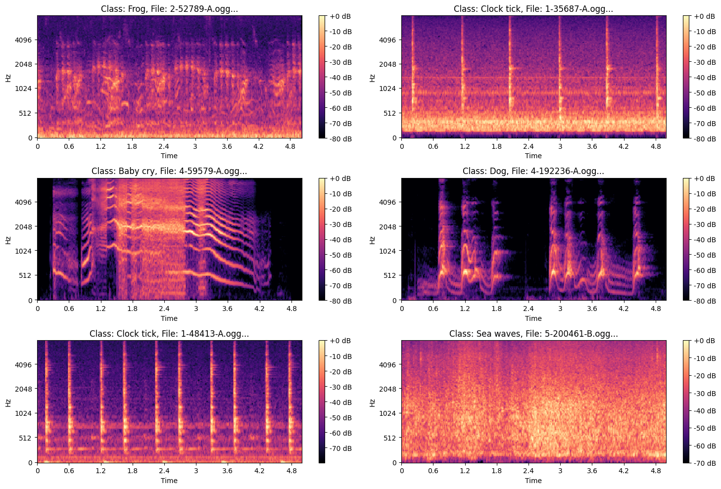
5. Mel Spectrogram Generation

Each cleaned audio chunk is transformed into a Mel spectrogram:

S = librosa.feature.melspectrogram(
    y=y, sr=SR,
    n_fft=N_FFT,
    hop_length=HOP_LENGTH,
    n_mels=N_MELS
)
S_dB = librosa.power_to_db(S, ref=np.max)

Output: 128×128 PNG images
Separate directories per class
Supports both original & augmented samples

These images become the CNN input.

Example of Mel Spectrogram Images

6. Dataset Validation

After spectrogram creation:

Corrupted images removed
Duplicate hashes filtered
Filename integrity checked
Class folders validated

df['file_hash'] = df['full_path'].apply(get_hash)
duplicate_hashes = df[df.duplicated(subset=['file_hash'], keep=False)]

This step ensures clean, reliable training data.

7. Building TensorFlow Datasets

The dataset is built with batching, caching, prefetching:

train_ds = tf.data.Dataset.from_tensor_slices((train_paths, train_labels))
train_ds = train_ds.map(load_and_preprocess, num_parallel_calls=AUTOTUNE)
train_ds = train_ds.shuffle(1024).batch(batch_size).prefetch(AUTOTUNE)

I used a simple image-level augmentation pipeline:

data_augmentation = tf.keras.Sequential([
    tf.keras.layers.InputLayer(input_shape=(231, 232, 4)),
    tf.keras.layers.RandomFlip("horizontal"),
    tf.keras.layers.RandomRotation(0.1),
    tf.keras.layers.RandomZoom(0.1),
])

8. CNN Architecture

The CNN captures deep frequency-time patterns across Mel images.

Key features:

Multiple Conv2D + BatchNorm blocks
Dropout
L2 regularization
Softmax output

model = Sequential([
    data_augmentation,
    Conv2D(32, (3,3), padding='same', activation='relu', kernel_regularizer=l2(weight_decay)),
    BatchNormalization(),
    MaxPooling2D((2,2)),
    Dropout(0.2),
    # ... more layers ...
    Flatten(),
    Dense(num_classes, activation='softmax')
])

9. Training Strategy

reduce_lr = ReduceLROnPlateau(monitor='val_loss', factor=0.5, patience=10)
early_stopping = EarlyStopping(monitor='val_loss', patience=40, restore_best_weights=True)

history = model.fit(
    train_ds,
    validation_data=val_ds,
    epochs=50,
    callbacks=[reduce_lr, early_stopping]
)

The model converges smoothly while avoiding overfitting.

10. Evaluation

Performance is evaluated using:

Accuracy
Precision, recall, F1-score
Confusion matrix
ROC/AUC curves

y_pred = np.argmax(model.predict(test_ds), axis=1)
print(classification_report(y_true, y_pred, target_names=le.classes_))

Confusion matrix:

sns.heatmap(confusion_matrix(y_true, y_pred), annot=True, cmap='Blues')
plt.title("Confusion Matrix")
plt.show()

11. Saving the Model & Dataset

model.save("Audio_Model_Classification.h5")
shutil.make_archive("/content/spectrograms", 'zip', "/content/spectrograms")

The entire spectrogram dataset is also zipped for sharing or deployment.

Final Notes

This project demonstrates:

How to clean & prepare raw audio at a professional level
Audio augmentation best practices
How Mel spectrograms unlock CNN performance
A full TensorFlow training pipeline
Proper evaluation, reporting, and dataset integrity

If you're working on sound recognition, speech tasks, or environmental audio detection, this pipeline gives you a complete production-grade foundation.

Results

Note: Click the image below to view the video showcasing the project’s results.

Note: If the video above is not working, you can access it directly via the link below.

Watch Demo Video

Downloads last month: -; Downloads are not tracked for this model. How to track

AIOmarRehan
/

CNN_Audio_Classification_Model_with_Spectrogram